 This image show the "true colour" version, with the blue range
assigned to the blue colour, green range to green colour and red range
to red colour.
This image show the "true colour" version, with the blue range
assigned to the blue colour, green range to green colour and red range
to red colour.Assigment 8 in GEG2210 - Data Collection - Land Surveying, Remote Sensing and Digital Photogrammetry
By Petter Reinholdtsen and Shanette Dallyn, 2005-05-01.
This exercise was performed by logging into jern.uio.no using ssh and running ERDAS Imagine. Started by using 'imagine' on the command line. The images were loaded from /mn/geofag/gggruppe-data/geomatikk/
We tried to use svalbard/tm87.img, but it only have 5 bands. We decided to switch, and next tried jotunheimen/tm.img, which had 7 bands.
The pixel values in a given band is only a using a given range of values. This is because sensor data in a single image rarely extend over the entire range of possible values.
The peak values of the histograms represent the the spectral sensitivity values that occure the most often with in the image band being analysed.
This image show the "true colour" version, with the blue range
assigned to the blue colour, green range to green colour and red range
to red colour.
 Water acts as an absorbing body so in the near infrared spectrum,
water features will appear dark or black meaning that all near
infrared bands are absorbed. On the other hand, land features
including ice, act as reflector bodies in this band. The histogram
show most values between 7 and 110. The mean is 40.1144. There are
two peaks at 7 and 40.
Water acts as an absorbing body so in the near infrared spectrum,
water features will appear dark or black meaning that all near
infrared bands are absorbed. On the other hand, land features
including ice, act as reflector bodies in this band. The histogram
show most values between 7 and 110. The mean is 40.1144. There are
two peaks at 7 and 40.


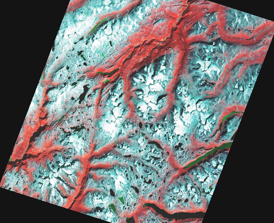
Comparing a map we found on the web, and the standard infrared image composition, we can identify some features from the colors used:

Next, we tried to shift the frequencies displayed to use blue for the red band, green for the near ir band and red for the mid ir (1.55-1.75 um). With this composition, we get some changes in the colours of different features:
We also tried to do histogram equilization on the standard infrared composition. This changed the colours in the image, making the previously green areas red, and the brown areas more light blue. In this new image, we can clearly see the difference between two kind of water, one black and one green. We suspect the green water might be deeper, but do not know for sure.
We decided to work on the grey scale version of the thermal infrared. This one has lower resolution then the rest of the bands, with 120m spatial resolution while the others have 30m spatial resolution.
The high pass filtering seem to enhance the borders between the pixels. Edge detection gave us the positions of glaciers and water. We tried a gradient filter using this 3x3 matrix. The matrix was chosen to make sure the sum of all the weights were zero, and to make sure the sum of horizontal, vertical and diagonal numbers were zero too.
| 1 | 2 | -1 |
| 2 | 0 | -2 |
| 1 | -2 | -1 |
It gave a similar result to the edge detection.
We also tried unsharp filtering using this 3x3 matrix, selected also to make sure the sum of all the weights were zero, and making sure the high frequency changes had extra weight.
| -1 | -1 | -1 |
| -1 | 8 | -1 |
| -1 | -1 | -1 |
This gave similar results to the edge detection too.
We started to suspect that the reason the 3x3 filters gave almost the same result was that the fact that the spatial resolution of the thermal band is actually 4x4 pixels (120 m, while the pixel size was 30m). Because of this, we tried with a 5x5 matrix, making sure it sums up to 0.
| -1 | -1 | -1 | -1 | -1 |
| -1 | -1 | -1 | -1 | -1 |
| -1 | -1 | 24 | -1 | -1 |
| -1 | -1 | -1 | -1 | -1 |
| -1 | -1 | -1 | -1 | -1 |
 Next, we tried some different weight:
| -1 | -1 | -1 | -1 | -1 |
| -1 | -2 | -2 | -2 | -1 |
| -1 | -2 | 32 | -2 | -1 |
| -1 | -2 | -2 | -2 | -1 |
| -1 | -1 | -1 | -1 | -1 |
This one gave more lines showing the borders between the thermal pixels. See the included image.